The Structure Is the Asset
Introduction
Ask whether a business should train its models on an ontology instead of on classic static data, and the honest answer starts by correcting the question. An ontology is not an alternative to data. It is data that can keep what a static export throws away: which records are the same customer across systems, how they connect, what was true as of each moment, what a code means when two systems name it differently, and which decisions were made and what followed. Our reading of the research is that this is where the value sits: in the structure, not in the model. A disclosure up front, because it bears on how you read this: Ardenus sells an ontology layer for field-service operators, so a conclusion that the structure is the asset is seller-convenient. Weigh it accordingly. Several of the strongest studies in this field carry vendor ties of their own, and we name them as we go.
- It is possible, with published methods. Graph models train directly on a keyed, time-stamped database, and hierarchies and rules can be built into a model. As far as our search found, no published study tests any of it on field-service data, so the mechanisms transfer and the magnitudes do not.
- The gain is in what the model can see. A model that sees linked, time-correct history often beats one that sees only the customer’s own row by a wide margin, and each new question gets far cheaper to answer. Most of that evidence comes from a system of record’s own keyed database, not an ontology layer.
- Language models should look up what changes. In our reading, fine-tuning a language model on a business’s changing facts is the weakest version of the idea. In controlled studies, writing stable knowledge out in many forms has helped.
- The ontology is not the alpha. In our reading, a layer sold to every competitor is table stakes, and the edge comes from what the structure makes cheap, keeps, and learns from your own decisions, faster than rivals copy it. It is a rate more than a stock.
What training on an ontology means
Training on an ontology is not one technique but several, and the evidence behind each differs sharply. By “ontology” we mean what we described in the data foundation beneath enterprise AI: a shared, machine-readable model of the business, its entities and how they relate, which for training this essay also asks to keep what was true as of each moment and which decisions were made.
| When | What the ontology does | Strength of the evidence (our assessment) |
|---|---|---|
| Before training: building the training set | Joins records along real relationships, rebuilds each feature as of the moment of prediction, maps different systems’ codes to shared concepts, and turns business rules into labels (the joins and as-of features need only a system of record’s own keys and timestamps, where it keeps history) | Strongest |
| During training, for models trained from scratch | Lets a graph model learn on the entity graph directly, or builds a hierarchy into the model | Real but conditional: largest where the signal sits in linked records, or where data is thin |
| Language-model pretraining | Generates varied training text from the graph’s facts | Works for stable knowledge on a niche corpus |
| Language-model post-training (fine-tuning) | Trains a model on question-and-answer pairs from the graph | Weakest when the facts change |
| After training: at decision time | Supplies current facts and records each decision and its outcome as the next round’s labels | The part that compounds, if decisions vary enough |
Most of what a field-service operator would train, such as models that predict cancellations, callbacks, job durations or collections risk, is trained once, from scratch, with no separate pretraining and post-training stage. That is why, in our reading, most of the value lands before and during training.
The right comparison has three rungs, not two: an export of each entity’s own row with today’s values; the system of record’s own keyed database, which relational methods can use directly wherever its tables carry timestamps; and an ontology layer over one or more such systems. Most of the evidence below measures the step from the first rung to the second. What the third adds, for a multi-branch operator, rests on thinner evidence: identity across acquired systems, the subject of entity resolution as a decision; history kept where the record overwrites, which can live in the record itself or in a layer, the subject of the system of record forgets; concepts that mean the same thing across vendors; and decisions stored as records.
Same model, more of the record
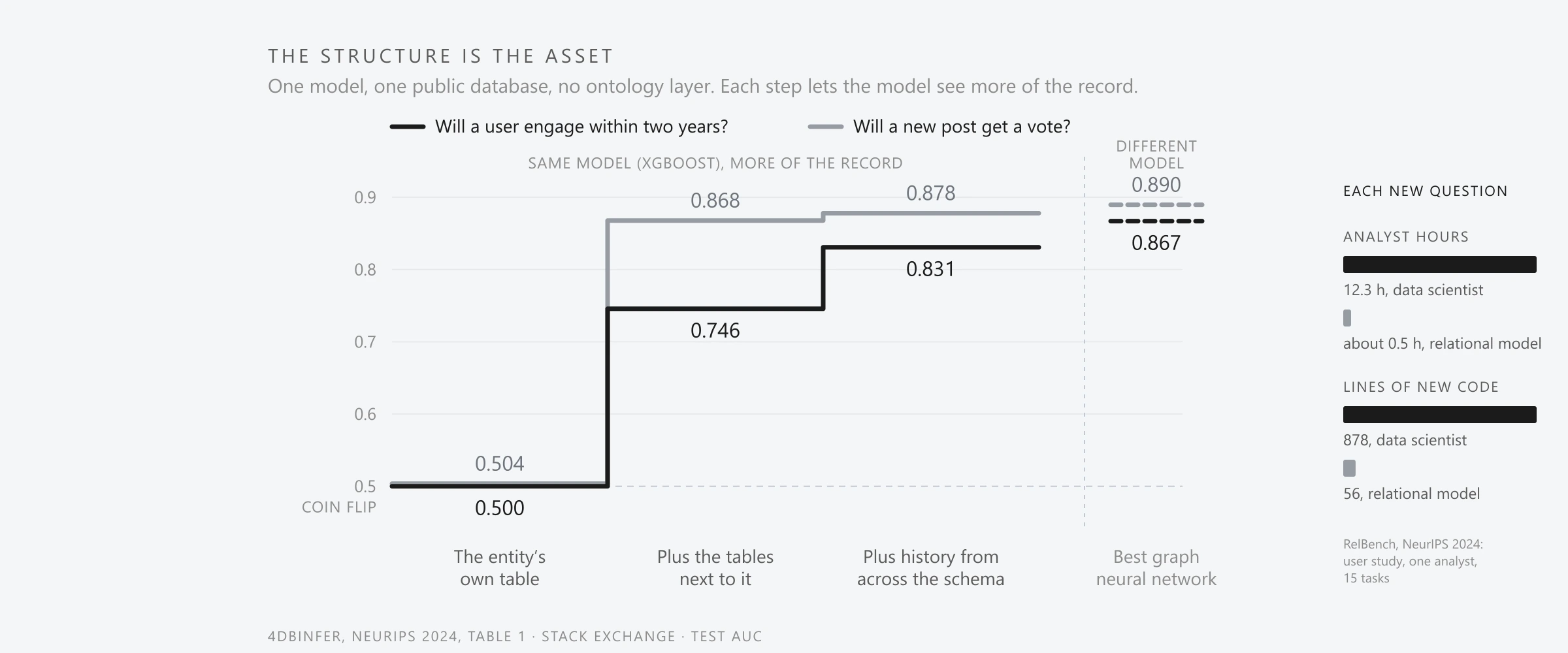
The cleanest test holds the model fixed and changes only what it can see. 4DBInfer, an Amazon-led benchmark published at NeurIPS 2024, does this on a Stack Exchange database, and the chart at the top of this page plots it. Asked whether a user will vote, comment or post in the next two years, XGBoost trained on the user’s own table scores 0.500 AUC, a coin flip. Every model the benchmark tried on that table alone scored the same, so this rung is a floor, not a picture of a good customer export. Given the adjacent tables, the same model scores 0.746; given history aggregated across the whole schema by deep feature synthesis, 0.831. The best graph neural network, a model that learns from the network of linked records directly, reaches 0.867. Holding the model fixed, the widening record covers 67 percent and then 90 percent of the distance from the coin flip to the graph model. On a second question, whether a new post gets a vote within a year, the adjacent tables alone go from 0.504 to 0.868, 94 percent of the way. The authors call these comparisons preliminary.
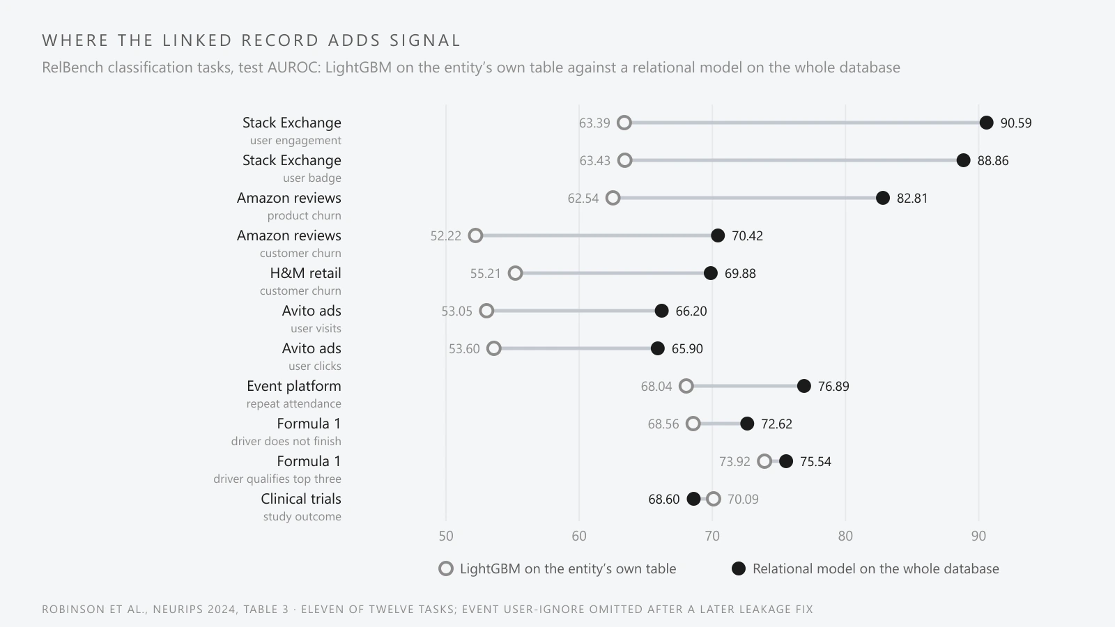
For breadth, RelBench, a NeurIPS 2024 benchmark from Stanford and Kumo.AI, where seven of its twelve authors list Kumo.AI, a company that sells this approach, compares LightGBM on the target entity’s own table with a relational graph model on the whole database across twelve classification tasks, scored from 0 to 100. The averages are 63.66 against 75.83, and the per-task gap runs from -1.49 to 27.20 points. Where the gap closes, the reason is instructive: predicting a clinical trial’s outcome, the single table did as well, because “This task has extremely rich features in the target table (28 columns total)”. The signal has to live in the linked records for linking them to pay.
Increasingly, it does not take a graph model either. A training-free method presented at ICML 2026, from the University of Hong Kong and Shanghai X-Lab, pairs SQL aggregations with an off-the-shelf tabular model and, on RelBench’s classification tasks with two leakage-suspect databases set aside, is in its authors’ words “the only RDB foundation model that is competitive with the fully supervised RelGT approach”, a graph model trained for each dataset. Our reading is that both camps work along the keys and timestamps the schema defines: the tabular methods flatten them, the graph models traverse them. The results argue against needing a particular model, not against needing the structure.
A sharper qualification concerns meaning. A peer-reviewed study that removed or distorted the knowledge graph in ten recommenders found that doing so “does not necessarily decrease recommendation accuracy, even for cold-start users”. One of the ten is the model behind the knowledge-graph lift cited in our essay on the regimes of prediction, so this qualifies that figure, though that model’s cold-start accuracy on one book dataset did fall more visibly. Our reading is that a recommender does not always use the knowledge it is given, so a graph’s meaning is not automatically where its lift comes from.
The labor dividend
In the one study that measures both, the clearer gain is not accuracy. In RelBench’s user study, one experienced data scientist built features by hand in SQL and tuned a LightGBM model on fifteen tasks. The relational model, which the authors call relational deep learning (RDL), matched or outperformed the data scientist on 11 of 15 tasks, though the authors, who applied a “boosting” step to it, are candid that “Even with boosting, the data scientist model outperforms RDL in several cases.” The larger difference was effort. Marginal time per new task fell from 12.3 hours to about half an hour, 96 percent less, and new code fell from 878 lines to 56, 94 percent less. The caveats matter: one analyst, a capped and non-iterative protocol, and, in the authors’ words, “this measures marginal effort, i.e., it does not include reusable code that can be amortized over many tasks”, nor the cost of building the clean database the method assumes.
Nor was the analyst’s baseline a static export. For the two churn tasks whose released feature code we inspected, it computes each feature as of the label’s timestamp, so the finding that a careful data scientist roughly ties the model is a statement about a time-correct feature table, which an export of today’s values cannot reproduce at past dates. The relational model used no ontology layer, only a clean, keyed database, so this dividend belongs to the second rung; our inference is that a layer’s part is supplying such a database where acquired systems do not share one.
Our inference, which no study measures, is that the dividend scales with the number of distinct questions asked of one structure: renewal risk, the shape of churn, callbacks, job duration, collections, and when demand arrives. One model does not justify it. A portfolio of them might.
Honest numbers often go down
A static snapshot fails in two ways: it ages, and it leaks. Vela and colleagues “observed temporal model degradation in 91% of cases” across four standard model types on 32 time-stamped datasets, a curated sample, so 91 percent is a rate within it, not a base rate. Leakage is the subtler failure: information that would not have been available at the moment of prediction finding its way into training. Kaufman, Rosset and Perlich, who formalized it, write that where only past information counts, “Legitimacy tagging is implemented by timestamping every observation.” They warn that database updates “are usually not timestamped and not stored separately”.
Fixing it often lowers the number, or changes which model wins. At one academic medical center, a widely deployed sepsis model scored an AUROC of 0.87 using all of its predictions up to discharge, 0.62 using only predictions made before patients met sepsis criteria, and 0.47 before clinicians’ first treatment order or sepsis test, such as a lactate measurement or blood culture. The authors attribute the drop to the model’s reliance on treatment indicators, which are clinicians’ own decisions, combined with less data being available early in a stay; a simpler model without clinician-order features also fell, from 0.60 to 0.51. In wound-care records the honest number rose slightly, but evaluating on the most recent data erased the advantage that complex ensembles showed under a random split. For an operator, a cancellation model fed a reason code, a logged save attempt or today’s balance can look brilliant in testing and fail in use.
That fix does not require an ontology: timestamps and an as-of join, which attaches each feature’s value as it stood at the moment of prediction, suffice. Our reading is that an ontology is the container that can make as-of the default rather than per-model hygiene, if it keeps time-versioned records; a feature store is another. The deeper point is timing. History that was never captured cannot be rebuilt, so an operator that keeps overwriting cannot buy it back later.
Where the ontology teaches
Meaning earns its keep when the systems underneath a model change. When a hospital switched electronic-record software in 2008, the same measurement got a new code. On raw codes, a random forest’s mortality AUROC fell by up to 0.29; grouping 181 raw item codes into 68 expert-defined clinical concepts held the worst drop to 0.06. The concepts were hand-built for that database; an automatic mapping to a formal medical ontology did not rescue the random forest or a recurrent network. The operator’s version is a branch changing systems after an acquisition, the subject of the post-acquisition system decision. Shared concepts make models portable without erasing the differences between sites: a sepsis model trained on harmonized data from four intensive-care databases scored an AUC of 0.846 on held-out patients from its own sites, 0.761 at other sites, and 0.807 after fine-tuning on 10 percent of each new site’s data.
Built into the model itself, an ontology pays mostly where data is thin. Representing each diagnosis code through its ancestors in a medical ontology raised a top-20 accuracy measure on codes in the 20th to 40th percentile of training frequency from 0.0731 to 0.1787, though most of that lift needed an extra initialization learned from which codes appear together: the ontology alone reached 0.1016, and simply replacing each code with its parent beat it. The most transferable result is forecasting. Forcing forecasts to add up across a hierarchy of 555 tourism series cut the average error of ARIMA forecasts by 12.4 percent for national totals by purpose of travel and 6.4 percent for states, with smaller gains from better base forecasts. A branch, region and company forecast that has to add up is the operator’s version.
A wrong ontology can do worse than none. A randomly generated hierarchy scored below the plain baseline it was meant to improve at most data sizes, so the prior is only as good as the curation behind it, which ties this evidence to the cost of dirty data. That also answers the strongest objection, Sutton’s “bitter lesson” that building in human knowledge “always helps in the short term” and then loses to general methods that scale with computation. Our reading is that the evidence agrees: knowledge injected as a human prior fades as data grows, while structure kept as data, the keys, links and timestamps, is what general learners consume.
Decisions become labels, if you log them
What a static export typically loses, and a living structure can hold, is which decision was made and what followed. Learning from your own decisions has worked where the decisions were varied at random and feedback was fast. Microsoft’s Decision Service, in a first-party preprint, reported a click-through gain of more than 25 percent over two weeks on one section of MSN, 5.3 percent on a higher-traffic one, and more than 30 percent over editorial ranking on another site. The value depends on discipline. When the team injected common logging failures into one day of MSN data, such as recording an overridden action or leaking the decision into the features, the estimate of a policy’s performance “deviated from its performance during testing, by a factor ranging from 1.2x to 8.7x”, where testing was itself an offline estimate on held-out logs from the same day, against within 5 percent with correct logs.
Learning a better decision rule from logs without experiments needs everything that drove the decision to be recorded, with every kind of case having had a real chance of each action, or something that varies the decision as if at random. A deterministic dispatch rule gives a learner nothing to compare. Outcomes are also selectively observed. In New York City pretrial decisions, Kleinberg and colleagues trained on 221,876 cases from an analysis sample of 758,027, with outcomes visible only for released defendants. At the judges’ jailing rate, an algorithmic rule could cut failure to appear by between 14.4 percent, a worst case that treats every jailed defendant as certain to fail, and 24.7 percent, which assumes the judges saw nothing relevant that the data did not record. Field service has the same shape: pest activity is seen only where a technician inspected.
An ontology can also supply labels directly through weak supervision, labels produced by rules and reference data rather than by hand. On four relation-extraction tasks, Snorkel’s authors report that it beat labels from a knowledge base alone by 15.9 to 38.8 F1 points on the three tasks where a knowledge base applied, and a regular-expression baseline by 9.2 points on the fourth. But on eight English text benchmarks whose weak labels came mostly from simple rules, that kind of edge is “mostly wiped out” once a few clean labels can be trained on.
Teach the structure, look up the facts
Language models are where “training on an ontology” is most often imagined, usually as fine-tuning, and where the evidence is most mixed. For stable facts, restatement helps. In a controlled study of synthetic biographies of 100,000 fictional people, a GPT-2-size model pretrained on one fixed-format biography per person and then fine-tuned on questions about half of them answered questions about the other half 9.7 percent of the time; five differently worded, shuffled biographies raised that to 96.6 percent, and varied wording without shuffling reached 41 percent. Generating synthetic text about the entities in a 1.3-million-token niche corpus, with the entities drawn from the documents by a GPT-4 model rather than from a curated graph, raised closed-book accuracy from 39.49 to 56.22 percent, more than 80 percent of what retrieval added.
For facts that change, the evidence points the other way. As a model learns fine-tuning examples carrying facts it did not know, they “linearly increase the model’s tendency to hallucinate”. In that study of one model, PaLM 2-S, a training set made only of unfamiliar facts dropped test accuracy from 37.5 at early stopping to 25.8 at convergence, though stopping early largely avoided the harm. Retrieval beat unsupervised fine-tuning in 28 of 30 settings of a knowledge benchmark, and on current events, fine-tuning one model cut its accuracy from 0.353 to 0.219.
Our reading is that the evidence supports a division of labor: the model’s weights for what is stable, such as the business’s vocabulary, relation types and procedures, and retrieval for what changes, such as today’s route, a balance, a status or a price. That half is covered in grounding and the reliability of AI and the diminishing returns of context.
Where the alpha comes from
In finance, alpha is the return above what a benchmark pays for the risk taken. Its literature is a useful analogy, though none of its magnitudes transfer to a service business. Grossman and Stiglitz showed that when information is costly to acquire, prices reflect it “but only partially, so that those who expend resources to obtain information do receive compensation”. That is compensation for a cost, not a free rent: in their equilibrium the informed are no better off once the cost is paid. Stock prices were slow to reflect news about a firm’s principal customers even though those links were public, and a value-weighted long-short strategy on the lag earned a three-factor alpha of about 1.55 percent a month from 1981 to 2004, before trading costs. Such edges decay. Across 97 published predictors, “Portfolio returns are 26% lower out-of-sample and 58% lower post-publication.” Our reading of the mechanism, not the numbers: an edge exists where processing is costly and others skip it, and publication erodes it.
Business evidence on data is real but modest and conditional. Among about 18,000 manufacturing plants in Census data, those that adopted data-driven decision-making (DDD) between 2005 and 2010 had about 3 percent higher value added than non-adopters, but plants of multi-unit firms “show no significant differential in productivity due to DDD”, which we read as a caution for multi-branch operators. Across 814 public firms, the average gain from big-data systems became insignificant after correcting for reverse causality, surviving only in IT-intensive and highly competitive industries, and only when each is estimated separately.
Who captures the learning matters too. Hagiu and Wright argue that “In most instances people grossly overestimate the advantage that data confers.” Their formal model separates learning by pooling different customers’ data from learning from each customer’s repeated use. The winning firm earns more from pooled learning, while learning from repeated use leaves customers better off but builds a switching cost that grows over time. Read with the vendor as the firm and operators as its customers, which is our mapping, not the authors’: a vendor that pools learning across competing operators raises everyone’s floor, which genuinely helps an operator with thin history, but the moat is the vendor’s. By our analogy, not McLean and Pontiff’s, selling the same layer to every competitor is the publication event. An operator’s edge has to come from learning on its own customers, decisions and outcomes. Because that learning becomes a switching cost toward whoever holds the history, the operator should own its time-correct history and be able to take it elsewhere.
Our synthesis, labeled as such: the ontology is not the alpha. Together with the system of record’s own keys and timestamps, which supply much of each, it does three things. It lowers the cost of answering a question below what rivals pay, which is where the labor dividend shows up; that an edge needs a lower cost than rivals face is our extension of Grossman and Stiglitz, not their result. It keeps time-correct history that rivals cannot acquire after the fact. And it records decisions and outcomes, which become the business’s own training labels. Because practices diffuse, what lasts longest is the speed of the learning loop, a rate more than a stock. The stock still counts, but in a field experiment at a news site, an algorithm that beat human editors by about 2.5 percent in clicks on average turned to minus 9.5 percent during a week-long bug that froze personal-data updates. Where an operating edge shows up in a company’s price is the subject of valuation follows revenue quality.
What this means for the operator
So, should you train models on an ontology instead of static data? Train them on keyed, time-stamped structure, the system of record’s own where it keeps history and an ontology layer’s where it does not, and do not expect the model to be the advantage. Start keeping time-correct, event-level history now, because it cannot be bought later. Log each decision with the rule that chose it, its context, who decided and the outcome, and vary a little on purpose where that is safe and compliant. Map acquired systems to shared concepts before consolidating them, and expect to recalibrate each branch. Before buying graph models, test whether linked records share outcomes, such as callbacks clustering by technician beyond each customer’s own history. Score every model as of the moment of the decision, and keep changing facts out of model weights.
The limits are real. No study measures any of this in field service: our search of titles and abstracts in two applied operations journals from 2015 to 2026 found no paper testing whether churn, service time or callbacks cluster by technician, route or neighborhood. In production, the gain from graph structure itself is small. LinkedIn’s graph models added roughly 0.1 to 2.4 percent online on top of mature models, and Google Maps’ graph model gained about 0.2 to 2 percent over the strongest non-graph model on historical data and under 1 percent in live use, and as we argue in the limits of benchmarks as value signals, a benchmark win is not a production result. Published costs, such as a back-of-envelope estimate of roughly $2 to $6 per manually curated knowledge-graph fact, price hand-authoring knowledge about the world. Our reading is that an operator’s real costs are mapping, identity resolution, cleaning and keeping it current, and we found no study that prices them.
The disclosure from the top belongs here in full. Ardenus sells an ontology layer, so an essay concluding that the structure is the asset is seller-convenient, and a reader should weigh it that way. To be fair to the other side, much of the benefit needs no ontology at all: timestamps and as-of joins prevent leakage on their own, a careful, time-correct feature table leaves only a small accuracy gap to the relational models, and flat models win when the signal sits in an entity’s own row. On our mapping of Hagiu and Wright’s model, learning pooled across competing operators raises everyone’s floor without giving any operator an edge over another, and the advantage it builds accrues to the vendor. The supporting evidence carries vendor ties of its own, in RelBench (Kumo.AI) and 4DBInfer (Amazon). No result, saving, or metric is attributed to Ardenus here, no client or first-party data appears anywhere in this essay, and both charts transcribe published tables. You can read more of our research on the Ardenus articles hub, or see the platform itself on the technology page.
Sources and methodology
- RelBench: A Benchmark for Deep Learning on Relational Databases (Robinson et al., NeurIPS 2024 Datasets and Benchmarks; seven of twelve authors at Kumo.AI) - Table 3 and the user study: 11 of 15 tasks, 12.3 to about 0.5 hours, 878 to 56 lines of new code; the released user-study code.
- 4DBInfer: A 4D Benchmarking Toolbox for Graph-Centric Predictive Modeling on RDBs (Wang et al., NeurIPS 2024 Datasets and Benchmarks; Amazon) - Table 1, Stack Exchange user churn and post popularity.
- No Need to Train Your RDB Foundation Model (Xu et al., ICML 2026).
- KG4RecEval: Does Knowledge Graph Really Matter for Recommender Systems? (Zhang et al., ACM TOIS 2025).
- Temporal Quality Degradation in AI Models (Vela et al., Scientific Reports 2022).
- Leakage in Data Mining: Formulation, Detection, and Avoidance (Kaufman, Rosset and Perlich, KDD 2011).
- Evaluation of Sepsis Prediction Models before Onset of Treatment (Kamran et al., NEJM AI 2024).
- Implications of Non-stationarity on Predictive Modeling Using EHRs (Jung and Shah, Journal of Biomedical Informatics 2015).
- Feature Robustness in Non-stationary Health Records: Caveats to Deployable Model Performance in Common Clinical Machine Learning Tasks (Nestor et al., MLHC 2019).
- Predicting Sepsis Using Deep Learning Across International Sites: A Retrospective Development and Validation Study (Moor et al., eClinicalMedicine 2023).
- GRAM: Graph-based Attention Model for Healthcare Representation Learning (Choi et al., KDD 2017).
- Optimal Forecast Reconciliation for Hierarchical and Grouped Time Series Through Trace Minimization (Wickramasuriya, Athanasopoulos and Hyndman, JASA 2019).
- The Bitter Lesson (Sutton, 2019, essay).
- Making Contextual Decisions with Low Technical Debt (Agarwal et al., arXiv 1606.03966, Microsoft, preprint).
- Human Decisions and Machine Predictions (Kleinberg et al., Quarterly Journal of Economics 2018).
- Snorkel: Rapid Training Data Creation with Weak Supervision (Ratner et al., PVLDB 2017).
- Weaker Than You Think: A Critical Look at Weakly Supervised Learning (Zhu et al., ACL 2023).
- Physics of Language Models: Part 3.1, Knowledge Storage and Extraction (Allen-Zhu and Li, ICML 2024).
- Synthetic Continued Pretraining (Yang et al., ICLR 2025).
- Does Fine-Tuning LLMs on New Knowledge Encourage Hallucinations? (Gekhman et al., EMNLP 2024).
- Fine-Tuning or Retrieval? Comparing Knowledge Injection in LLMs (Ovadia et al., EMNLP 2024).
- On the Impossibility of Informationally Efficient Markets (Grossman and Stiglitz, American Economic Review 1980).
- Economic Links and Predictable Returns (Cohen and Frazzini, Journal of Finance 2008).
- Does Academic Research Destroy Stock Return Predictability? (McLean and Pontiff, Journal of Finance 2016).
- Data in Action: Data-Driven Decision Making in U.S. Manufacturing (Brynjolfsson and McElheran, U.S. Census Bureau CES Working Paper 16-06).
- The Effect of Big Data and Analytics on Firm Performance: An Econometric Analysis Considering Industry Characteristics (Müller, Fay and vom Brocke, Journal of Management Information Systems 2018).
- The Editor and the Algorithm: Recommendation Technology in Online News (Peukert, Sen and Claussen, Management Science 2024).
- When Data Creates Competitive Advantage (Hagiu and Wright, Harvard Business Review 2020) and Data-enabled Learning, Network Effects, and Competitive Advantage (Hagiu and Wright, RAND Journal of Economics 2023).
- LiGNN: Graph Neural Networks at LinkedIn (Borisyuk et al., KDD 2024).
- ETA Prediction with Graph Neural Networks in Google Maps (Derrow-Pinion et al., CIKM 2021).
- How Much Is a Triple? Estimating the Cost of Knowledge Graph Creation (Paulheim, ISWC 2018 Blue Sky Ideas track).